5 Standard Deviations is Always Unusual

Post #779

A definition of what is typical would be something which happens 95 times out of every 100 occasions. And, by definition, events that are atypical or unusual occur 5 or less times per 100 (5% of the time or less). When something which is variable distributes in a normal way, the center is the mean value and frequency is bell-shaped:

In this distribution of IQ scores, values rise as you go right, the mean value is 100, and a standard deviation away from the mean value is worth 15 points. 95% of all the scores show up within 2 standard deviations of the mean value of 100 — so that 95 of every 100 people who take an IQ test end up with IQ scores ranging from 70 up to 130.

But not all things which vary will vary according to this bell-shaped model. While being over 2 standard deviations from the mean is always unusual for IQ tests, in some distributions you have more than a 5% chance of being more than 2 standard deviations from the mean. Finding out what is unusual may require more work.

But there is a rule which works for every distribution of values: Chebychev’s theorem. In Chebychev’s theorem, there is a proof stating that the minimum portion of all values in a given population that is within k standard deviations of the mean will always — not sometimes, always — be at least as much as

\(1-\frac{1}{k^2}\)

With Chebychev theorem, it’s always the case that 5 standard deviations from the mean is unusual (i.e., <5% probable) and that over 20 standard deviations from the mean is so unusual that it demonstrates a “special cause” (variation due to common causes can’t explain values sitting beyond 20 standard deviations from a mean).

Real World Use

A real world application for this theorem would be to examine the historic reporting rate of serious adverse event reports (serious AERs) in the VAERS system for a mean reporting rate per million doses, and a standard deviation of the reporting rate.

Year … Net Doses (M) … serious AER … rate/M
1991 …… 127.818932 …………… 1,301 ………… 10.18
1992 …… 152.522129 …………… 1,441 ………… 9.45
1993 …… 170.365246 …………… 1,452 ………… 8.52
1994 …… 190.238536 …………… 1,545 ………… 8.12
1995 …… 145.786858 …………… 1,466 ………… 10.06
1996 …… 147.702015 …………… 1,455 ………… 9.85
1997 …… 166.13962 ….……….… 1,588 ………… 9.56
1998 …… 187.758677 …………… 1,673 ………… 8.91
1999 …… 202.176571 …………… 2,037 ………… 10.08
2000 …… 210.608388 …………… 2,006 ………… 9.52
2001 …… 202.266286 …………… 2,332 ………… 11.53

The mean rate of serious AERS is 9.62 per million net doses delivered. The standard deviation of the rate of serious AERS is 0.92 per million net doses delivered. The 99% upper bound on the standard deviation is 1.97 per million net doses delivered.

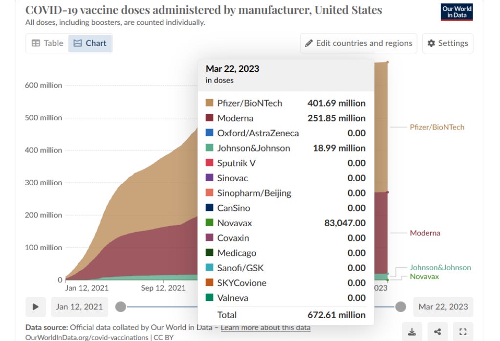
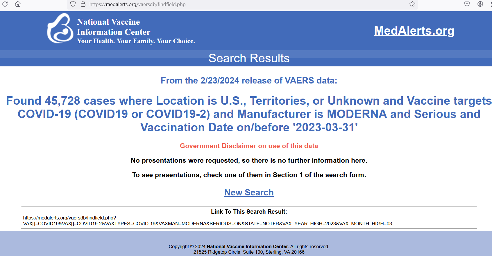
When the serious AER rate for Moderna is compared with these historic figures, the rate is so high (182 serious AERs per million doses) that — even using the 99% upper bound standard deviation — the Moderna serious AER rate is 87 standard deviations above the mean.

Because Chebychev’s theorem proves that a 5-standard-deviation shift is always unusual, and shifts over 20-standard-deviations demonstrate a special cause (common cause variation cannot explain shifts beyond 20 standard deviations; regardless of underlying distribution of values), data indicate that Moderna is especially harmful.

251.85 million doses by March 2023

45,728 Serious Adverse Event Reports by March 2023

182 serious AERs per million doses is a safety signal writ large, and may be historically unprecedented with regard to medical substances which have gained approval.

Reference

CDC. Surveillance for Safety After Immunization: Vaccine Adverse Event Reporting System (VAERS) --- United States, 1991--2001. https://www.cdc.gov/mmwr/preview/mmwrhtml/ss5201a1.htm

OurWorldInData. COVID-19 doses administered by manufacturer. https://ourworldindata.org/covid-vaccinations

MedAlerts VAERS Search Tool. https://medalerts.org/vaersdb/index.php