Bayes Model of Fetal Risk from Comirnaty
Post #1387

NOTE: An error was found in this post, and it has now been corrected.
As reported by two old geezers, taking Corminaty while pregnant is quite risky. To corroborate their findings, I used a Bayesian (Bayesian Twin Beta; or BTB) analysis. Here is their statistical analysis using Frequentist methods rather than Bayesian methods:
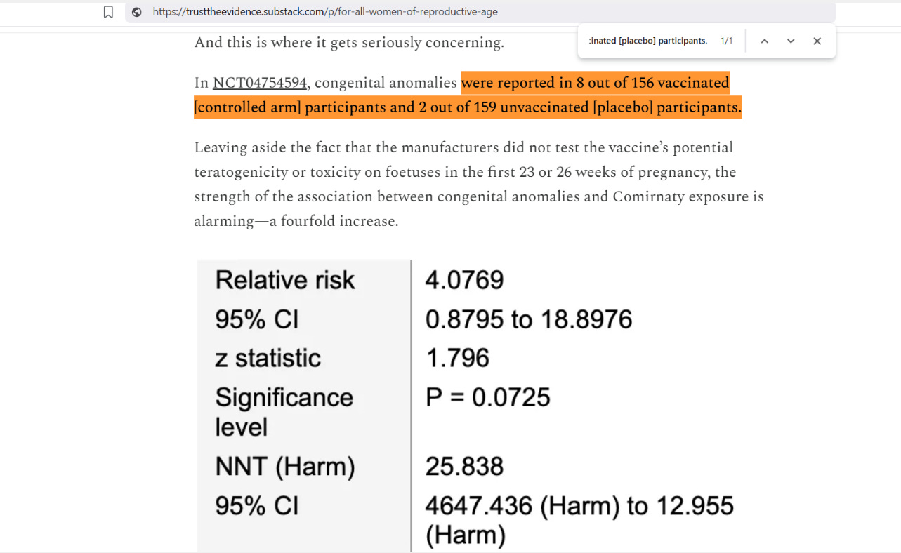
As you can see, congenital anomalies were found in the Comirnaty group at approximately 4x the rate that they were found in the unexposed placebo group. It is unfortunate that the original wording referred to the exposed Comirnaty group as being “controlled” — because control has a double-meaning here.
While the Frequentist method of analysis failed to uncover statistical significance from the findings, this is one of those times when a Bayesian method of analysis was able to get beyond the short-comings of a Frequentist method:
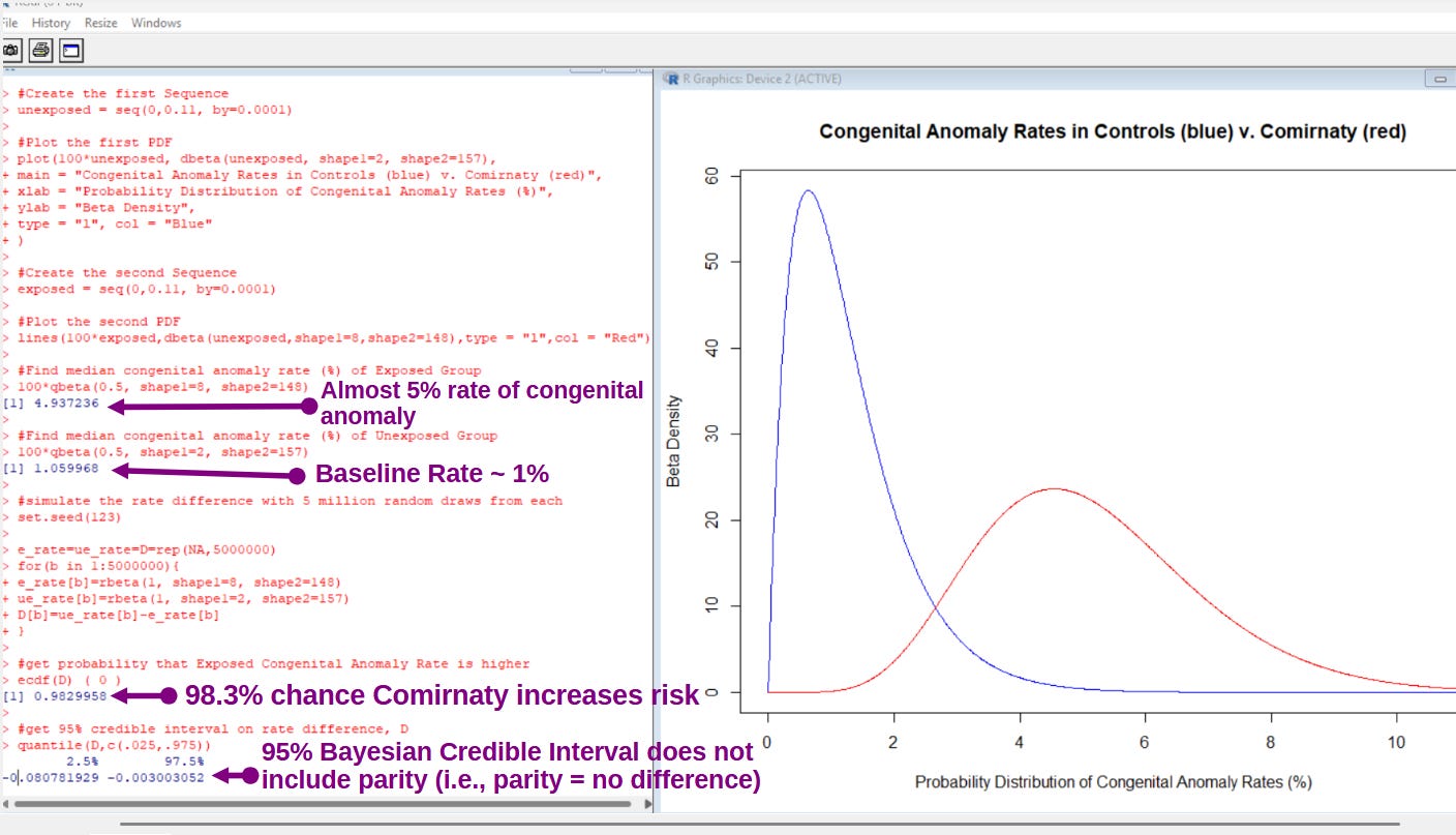
[click to enlarge]
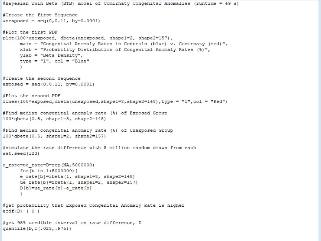
So that interested parties can perfectly replicate these findings, I’m including all of the code for the program (total run time ~ 49 seconds) below. After downloading R, then copy the code below and paste it into Notepad (or other basic word processor without any formatting). Open R and choose File > New Script and paste it into R.
Then highlight it all and hit Ctrl+R to run it — and after 49 seconds, watch the magic happen:
#Bayesian Twin Beta (BTB) model of Comirnaty Congenital Anomalies (runtime = 49 s)
#Create the first Sequence
unexposed = seq(0,0.11, by=0.0001)
#Plot the first PDF
plot(100*unexposed, dbeta(unexposed, shape1=2, shape2=157),
main = “Congenital Anomaly Rates in Controls (blue) v. Comirnaty (red)”,
xlab = “Probability Distribution of Congenital Anomaly Rates (%)”,
ylab = “Beta Density”,
type = “l”, col = “Blue”
)
#Create the second Sequence
exposed = seq(0,0.11, by=0.0001)
#Plot the second PDF
lines(100*exposed,dbeta(unexposed,shape1=8,shape2=148),type = “l”,col = “Red”)
#Find median congenital anomaly rate (%) of Exposed Group
100*qbeta(0.5, shape1=8, shape2=148)
#Find median congenital anomaly rate (%) of Unexposed Group
100*qbeta(0.5, shape1=2, shape2=157)
#simulate the rate difference with 5 million random draws from each
set.seed(123)
e_rate=ue_rate=D=rep(NA,5000000)
for(b in 1:5000000){
e_rate[b]=rbeta(1, shape1=8, shape2=148)
ue_rate[b]=rbeta(1, shape1=2, shape2=157)
D[b]=ue_rate[b]-e_rate[b]
}
#get probability that Exposed Congenital Anomaly Rate is higher
ecdf(D) ( 0 )
#get 95% credible interval on rate difference, D
quantile(D,c(.025,.975))
And here is how it looks inside of R:
Reference
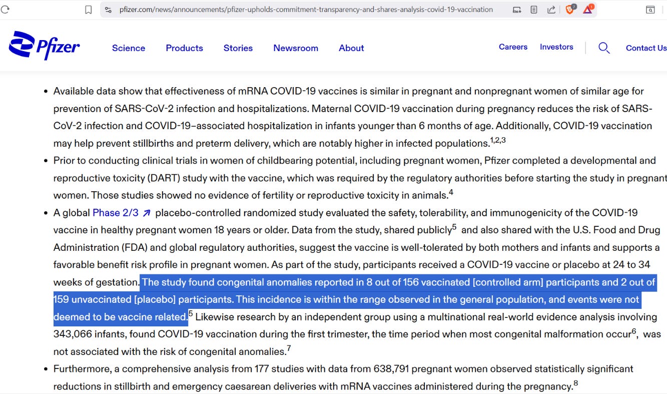
[Pfizer claims that having congenital anomalies in almost 5% of kids is “normal”] — https://www.pfizer.com/news/announcements/pfizer-upholds-commitment-transparency-and-shares-analysis-covid-19-vaccination